
二項ロジスティック回帰分析も目的変数は 1または0の配列です。Label Encoder で作成します。 このデータセットで社員の退職要因を分析する二項ロジスティック回帰分析をシリーズでブログしたいと思います。 Kaggle よりHRデータ のデータセットでオペレーションしました。
チートシート
| やりたいこと | 注意点 |
|---|---|
| 二項カテゴリカル・データを0/1の配列にする | Label Encoder を使う |
参照: sklearn.preprocessing.LabelEncoder
今回使うデータのポイント
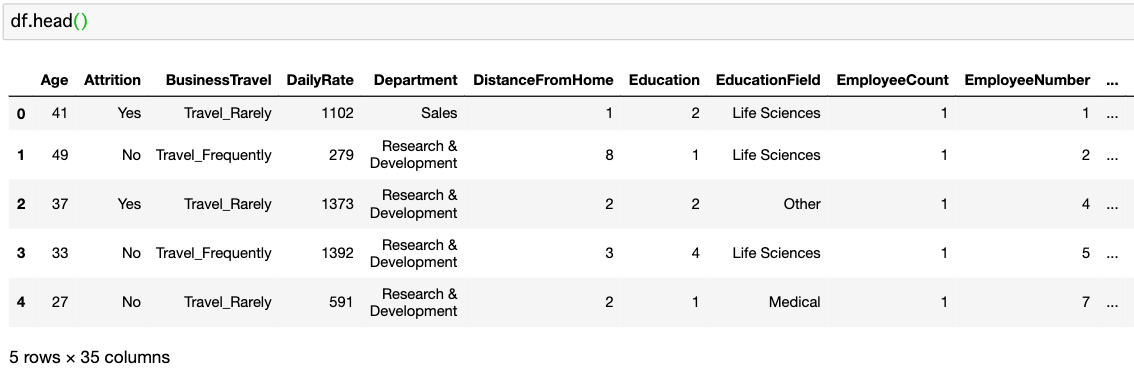
- 1,470名の社員の退職状況(attrition)に関する人事データ (Kaggleより)
- df.shape => 1470 x 35
- 目的変数用のデータフレームを作成します
サンプルデータセットについての記事で紹介しているHRデータです。
サンプルオペレーション
1
2
3
4
5
6
# Attrition に対してLabel Encodeし、最初の5行の結果をみる
from sklearn.preprocessing import LabelEncoder as LE
label_encoder = LE()
attrition_flag = df['Attrition']
attrition_encoded = label_encoder.fit_transform(attrition_flag)
attrition_encoded[0:5]
結果は以下のとおりです。 Attrition = Yes を1に、No を0にしています。
array([1, 0, 1, 0, 0])戻り値の配列をtarget_dfという名前のデータフレームにします。
1
2
3
# 1 = yes / 0 = no
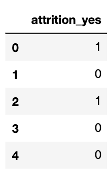
target_df = pd.DataFrame(attrition_encoded, columns=['attrition_yes'])
target_df.head()
計算結果のデータフレーム
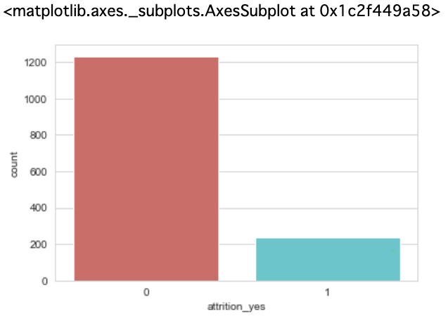
目的変数を可視化してみました
1
2
rcParams['figure.figsize'] = 6,4
sb.countplot(x='attrition_yes', data=target_df, palette='hls')
1
2
3
4
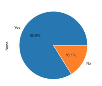
df_pie =target_df.groupby(by='attrition_yes').size()
labels = ['Yes', 'No']
plot = df_pie.plot.pie(y='attrition_yes', labels=labels, autopct='%.1f%%')
ひとこと
分類問題の基本である二項ロジスティック回帰分析のためのデータセット準備には、Label Encoderが必須アイテムです。また、作成した目的変数の可視化も合わせて行い、どんな割合で分類されているか確認しておきましょう。